The Machine Learning Primer: From fundamentals to a working app

A beginner-friendly guide to core ML concepts, practical techniques, and real-world implementation

September 6, 2025
21 min read

“Artificial Intelligence”, “Deep Learning”, “Machine Learning” (ML) are buzzwords that have been echoing all around us for the past decade. Most of us think we know what they mean. Or… do we?

I started questioning myself, trying to get a clearer understanding of these concepts and somehow ended up building a minimalistic machine learning model and simple ML application.

TLDR/video: A simple machine learning app that listens for voice commands. When it hears me saying the word “go”, it opens a web browser. All other words are ignored.

Let me share what I learned along the way.

Entering the world of Machine Learning

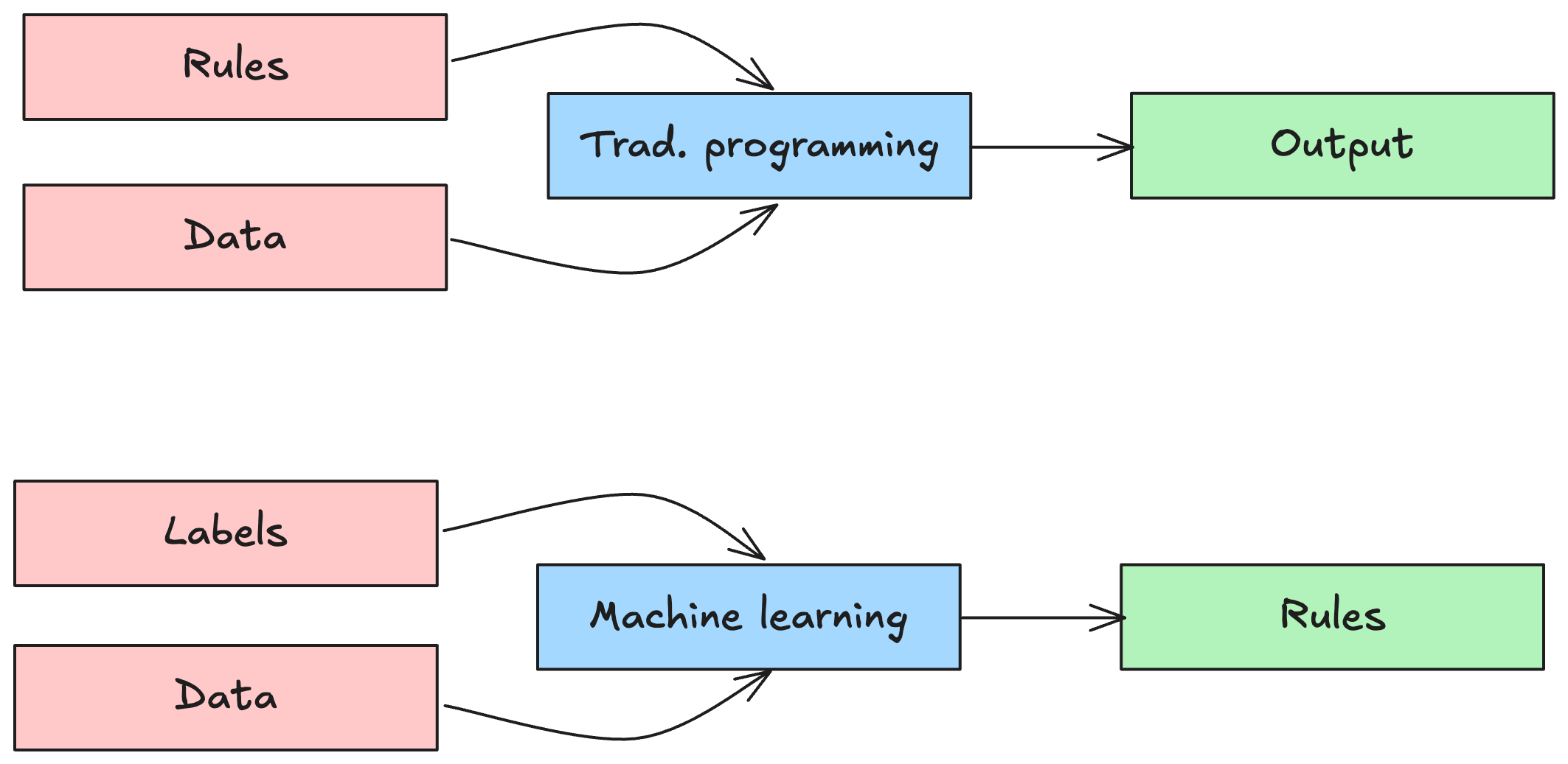
Machines that “think” aren’t exactly new. We’ve had devices like calculators for decades. They seem smart, they do math instantly, after all. But the truth is, they’re just really fast at following precise instructions. Everything they do is hard-coded and guaranteed: when you add 1 + 1, it will be 2. No doubts, no debate.

This is classic programming: deterministic, rule-based, and predictable.

Now, enter Machine Learning. Here, the game changes.

On contrary, machine learning has no exact algorithms and outcome is not precise. So why to bother? Machine learning shines when writing rules and algorithms would be overly complex if not impossible to define. E.g. to distinguish dog from a cat or to detect sarcasm in the sentence. Instead of giving the machine rules, we give it examples, lots of them, and let it figure out the patterns. We don’t program the model, we teach it to approximate outcome from a given input.

Let’s go back to the humble calculator. You give it some inputs, two numbers, and it gives you an output using the magical mathematical operation we call addition. Simple, right?

But let’s simplify even more. Instead of dealing with two numbers on input, imagine we take just one number and transform it into another using a bit of mathematical magic. In other words, we apply a function that maps input to output.

In ML, we define set of inputs and set of expected outputs. Expected output is oftentimes called a ground truth or target. In the context of data classification, you can also hear the term label which flags the data in input and output.

Example inputs and outputs:

x = [-1.0, 0.0, 1.0, 2.0, 3.0, 4.0] # input
y = [-3.0, -1.0, 1.0, 3.0, 5.0, 7.0] # ground truth

The learning process is all about figuring out the rule that takes us from X to Y. Ideally, the model will discover the underlying pattern, for example, that Y = 2X - 1 and then use that rule to make predictions for new inputs.

This is a trivial case. In the real world, things get messy. We often deal with complex, multi-dimensional inputs and outputs, images, text, sensor data, you name it. But let’s not go there just yet. For now, simple is good.

Let’s summarise the core of the Machine Learning:

Handles complex tasks
Scales well and handles well new unseen data
Improves by having new fresh data
Needs data (instead of explicit rules)
Probabilistic

Real world use cases

Machine learning is used across a wide range of fields, from video processing in self-driving cars, to language processing in the tools like ChatGPT, to predictive analytics in online trading. It powers anomaly detection in cybersecurity and fuels generative AI tools like DALL·E and MidJourney.

It is easy to assume that machine learning is always part of something big, like big data, big clouds, big models.

But ML isn’t just for massive servers and high-end GPUs. It’s also making its way into the world of microcontrollers, wearables for sports and health, and smart home devices, a trend known as TinyML. These are scenarios where the benefits of machine learning are needed, but resources like processing power, memory, or battery life are limited. In these cases, ML has to go on a diet and get smart without being power-hungry.

Basic Learning process

To demonstrate the learning process, we will use the same simple data set as before:

x = [-1.0, 0.0, 1.0, 2.0, 3.0, 4.0] # input
y = [-3.0, -1.0, 1.0, 3.0, 5.0, 7.0] # ground truth

We need to find or approximate the “rule” to get from X to Y. First, we need to choose a learning model, which is a mathematical structure that defines how inputs are mapped to the outputs.

In this simple case, let’s assume our best choice is a linear regression model which is represented by a linear function Y=w * X + b.

Here, w is called the weight, and b is the bias. Together, they define the line that our model uses to approximate the relationship between input and output.

There are much more complex learing models, than regression models, mainly:

Neural networks - a network of many parameters (weights, biases).
Decision trees - tree of rules.

Let’s stick with our simple linear regression model. The big question now is: how do we figure out the right values for w (weight) and b (bias) to make our function work?

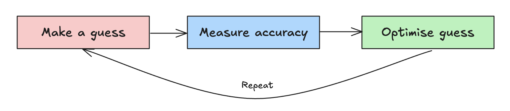
The answer? We guess.

Then we check how good the guess was. Then we guess again, but better this time. We repeat this process in a loop, gradually improving our guesses until the model is accurate enough.

In other words, we let the model learn by adjusting w and b step by step, aiming to reduce the error between its predictions and the actual values. This accuracy is usually measured with some kind of error metric, a score telling us how “bad” our guesses still are.

The following Python code tries a single manual guess of w and b. Our first guess is: w = 3 and b = 1 and we will calculate also how far we are from the ground truth, which represents the loss.

import math
import matplotlib.pyplot as plt

# Training data (optimal outcome: y=2x-1)
x = [-1.0, 0.0, 1.0, 2.0, 3.0, 4.0] # input
y = [-3.0, -1.0, 1.0, 3.0, 5.0, 7.0] # ground truth

# Guess the model (Y=w * X + b)
w = 3
b = 1

# Make a prediction
y_pred = []

for x_val in x:
    y_guess = x_val * w + b
    y_pred.append(y_guess)

print("Ground truth:", y)
print("Prediction:", y_pred)

# Calculate individual losses and overall loss using RMSE (Root Mean Squared Error).
individual_losses = []
print("\nIndividual Losses (Squared Errors):")
for i in range(len(x)):
    error = y_pred[i] - y[i]
    squared_error = error ** 2
    individual_losses.append(squared_error)

print(individual_losses)

# Calculate overall loss (Root Mean Squared Error)
mse = sum(individual_losses) / len(individual_losses)
rmse = math.sqrt(mse)
print(f"\nOverall Loss (Root Mean Squared Error): {rmse:.2f}")

...snipped...

As a result we got an array of predicted (guessed) Y values, which are slightly off the ground truth and the difference represent the loss:

Ground truth: [-3.0, -1.0, 1.0, 3.0, 5.0, 7.0]
Prediction: [-2.0, 1.0, 4.0, 7.0, 10.0, 13.0]

Individual Losses (Squared Errors):
[1.0, 4.0, 9.0, 16.0, 25.0, 36.0]

Overall Loss (Root Mean Squared Error): 3.89

The loss is calculated as Root mean squared error (RMSE). RMSE prevents negative losses cancellling out opposite ones. See this page to know more about the RMSE method. There are also others loss calculation methods - MAE (Mean Absolute Error), MSE (Mean Squared Error), etc.

Loss visualised: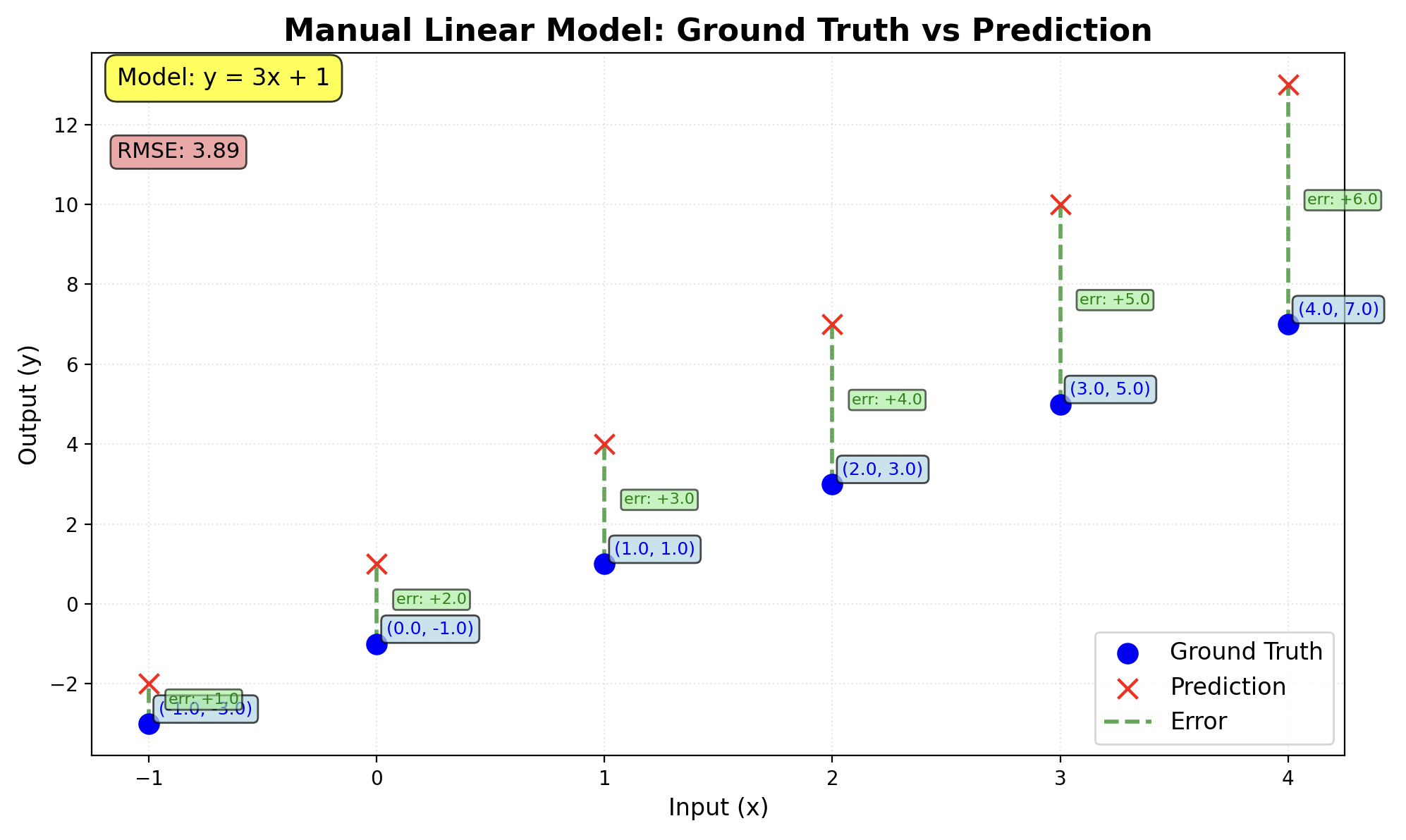

Our overall loss is 3.89 which is quite far from 0 (full precision). Our first guess was very wrong.

Impoved guessing by Gradient Descent learning

We can keep guessing and adjusting until the loss (the error in our predictions) gets low enough. But if we are working with large datasets, that trial-and-error approach could take forever.

Instead, we can be a bit smarter about our guesses. By observing how the loss changes when we tweak the weight and bias, we can adjust them more intelligently in the next round.

This clever trick is called Gradient Descent.

The simplest way to visualize it is as a smooth, symmetrical curve. Imagine you are standing on a hill (that hill represents the loss). Your goal is to walk downhill, step by step, until you reach the lowest point. That lowest point is where the loss is minimal and where our model is most accurate.

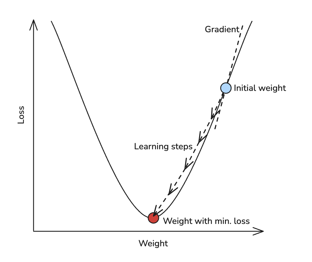
Gradient Descent helps us decide which way to step and how big each step should be, based on the shape of the hill beneath our feet.

To make Gradient Descent work, we need to keep track of a few important things:

How the loss is evolving after each guess?
How the gradient is changing (i.e. the difference in loss between the current and previous steps)?

Based on this information, we decide how much to adjust the weight in the next guess. This adjustment is called the learning rate (or learning step).

Here’s the tricky part:

If the learning rate is too large, we might overshoot the lowest point and bounce around without ever settling down.
If it is too small, the model will learn painfully slowly. It might take forever to get anywhere useful.

So, choosing the right learning rate is like choosing the right walking pace on that loss curve hill. Too fast? You trip and fall. Too slow? You never reach the bottom.

No worries, here comes the Tensorflow framework to save us!

Tensorflow

TensorFlow is a powerful library that allows data to “flow” through a series of computational operations. It can handle everything from simple scalars to 1D vectors, 2D matrices, and even complex multi-dimensional data structures.

To make things easier for us, TensorFlow also supports a handy tool called GradientTape (in Python, it is the tf.GradientTape class). This utility automates the Gradient Descent process by tracking the operations used to compute the loss and then calculating the gradients for us.

Here is a simple example of how to use Gradient Descent in Python with TensorFlow:

import tensorflow as tf
import matplotlib.pyplot as plt
import numpy as np

# Define our initial guess
INITIAL_W = 10.0
INITIAL_B = 10.0

# Define our simple regression model
class Model(object):
    def __init__(self):
        # Initialize the weights
        self.w = tf.Variable(INITIAL_W)
        self.b = tf.Variable(INITIAL_B)

    def __call__(self, x):
        return self.w * x + self.b

# Define our loss function
def loss(predicted_y, target_y):
    return tf.reduce_mean(tf.square(predicted_y - target_y))


# Define our training procedure
def train(model, inputs, outputs, learning_rate):
    with tf.GradientTape() as t:
        # loss function
        current_loss = loss(model(inputs), outputs)

        # Here is where you differentiate loss function w.r.t model parameters
        dw, db = t.gradient(current_loss, [model.w, model.b])  # dloss/dw, dloss/db

        # And here is where you update the model parameters based on the learning rate chosen
        model.w.assign_sub(learning_rate * dw)  # model.w = model.w - learning_rate*dw
        model.b.assign_sub(learning_rate * db)  # model.b = model.b - learning_rate*db
    return current_loss


# Define our input data and learning rate
xs = [-1.0, 0.0, 1.0, 2.0, 3.0, 4.0]
ys = [-3.0, -1.0, 1.0, 3.0, 5.0, 7.0]
LEARNING_RATE = 0.14

# Instantiate our model
model = Model()

# Collect the history of w-values and b-values to plot later
list_w, list_b = [], []
epochs = 50
losses = []

for epoch in range(epochs):
    list_w.append(model.w.numpy())
    list_b.append(model.b.numpy())
    current_loss = train(model, xs, ys, learning_rate=LEARNING_RATE)
    losses.append(current_loss)
    print('Epoch %2d: w=%.2f b=%.2f, loss=%.2f' %
          (epoch, list_w[-1], list_b[-1], current_loss))

Command output shows us, how each guess loop (called Epoch) and adjustment of weight and bias leads to the loss decrease:

Epoch  0: w=10.00 b=10.00, loss=715.67
Epoch  1: w=-6.19 b=3.56, loss=255.55
Epoch  2: w=3.74 b=5.72, loss=96.13
Epoch  3: w=-1.60 b=3.11, loss=39.55
Epoch  4: w=1.88 b=3.47, loss=18.51
Epoch  5: w=0.17 b=2.27, loss=10.01
Epoch  6: w=1.44 b=2.12, loss=6.13
Epoch  7: w=0.94 b=1.48, loss=4.08
...snipped...
Epoch 24: w=1.94 b=-0.82, loss=0.02
Epoch 25: w=1.95 b=-0.85, loss=0.01
Epoch 26: w=1.96 b=-0.87, loss=0.01
Epoch 27: w=1.96 b=-0.89, loss=0.01
Epoch 28: w=1.97 b=-0.90, loss=0.01
Epoch 29: w=1.97 b=-0.92, loss=0.00
...snipped...
Epoch 49: w=2.00 b=-1.00, loss=0.00

Our loss is 0.00, if weight is 2.00 and bias -1.00. We reached 100% accuracy. Which builds a rule Y=2X-1. 🎊

Easy, right?

Well… in the real world, things aren’t usually this simple.

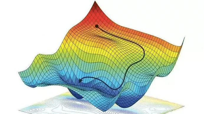
Instead of a single number as input (1-dimensional), real-world data often has dozens or even hundreds of dimensions. Once we move beyond 2 or 3 dimensions, things start to get tricky.

Even at just 3 dimensions, visualizing Gradient Descent becomes much harder. The “loss hill” we talked about earlier turns into a loss landscape with valleys, ridges, plateaus, and multiple local minima. Navigating through this terrain becomes a whole new challenge.

Neural networks

Now that we have covered regression models, it is time to take the next step: neural networks.

Neural networks are made up of interconnected computational units called neurons, which work together to discover relationships between our inputs (Xs) and outputs (Ys). When machine learning is powered by neural networks, it is often referred to as deep learning. These models can uncover complex patterns that simpler methods can’t easily capture.

What in neuron? The term neuron in neural networks is a metaphor - it represents a mathematical function. A simple example might look like this: Y = (w * X) + (...) + (...) + b. The more terms (brackets) we add to this function, the more neurons the network effectively has.

Each term in this function involves weights and inputs. In a neural network, the output from one layer becomes the input for the next.

Weights represent the connections between neurons in adjacent layers. More inputs and more neurons mean more connections — and therefore more weights.

Biases are tied to the number of neurons in a layer. Each neuron has its own bias, which modifies its output.

The simplest possible neural network consists of a single input, one neuron, and a single output:

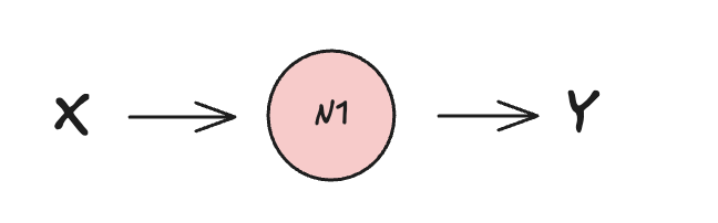
This setups results into single-layer neural network with single Y=(w * X) + b function processed by a single neuron.

We will use again the Gradient descent loss calculation. This time in combination with a so-called Dense neural network. For now it is sufficient to know, that Dense, or Fully connected neural networks are one of many types of neural networks.

Tensorflow offers abstraction API keras for building and training neural networks used in the (following code)[https://github.com/jkosik/jkosik.github.io/blob/main/_extra/ml/3_ml-tf-keras.py]:

import tensorflow as tf
from tensorflow import keras
import numpy as np

# Define the model
model = keras.Sequential([
    keras.layers.Dense(units=1, input_shape=[1]) # 1 neuron, 1 input
])

# Compile the model
model.compile(optimizer='sgd', loss='mean_squared_error') # stochastic gradient descent (sgd) and measure the loss as MSE

# Training data (y=2x-1)
xs = np.array([-1.0, 0.0, 1.0, 2.0, 3.0, 4.0], dtype=float) # input
ys = np.array([-3.0, -1.0, 1.0, 3.0, 5.0, 7.0], dtype=float) # ground truth output


# Train the model
model.fit(xs, ys, epochs=50) # make a guess, measure the loss, optimise and repeat epoch-times

# Make a prediction (runs the input through the trained model.)
print(model.predict(np.array([10.0]))) # try to predict the output of 10.0

The single neuron learn relation between X and Y and tries to predicts Y for X=10 and results in:

...snipped...
Epoch 48/50
1/1 ━━━━━━━━━━━━━━━━━━━━ 0s 16ms/step - loss: 0.2339
Epoch 49/50
1/1 ━━━━━━━━━━━━━━━━━━━━ 0s 18ms/step - loss: 0.2291
Epoch 50/50
1/1 ━━━━━━━━━━━━━━━━━━━━ 0s 17ms/step - loss: 0.2244
1/1 ━━━━━━━━━━━━━━━━━━━━ 0s 21ms/step
[[17.614405]]

Previously, our linear regression model (Y = 2X - 1) gave a precise result of 19. In contrast, our minimalistic neural network produced a result of 17.614405.

In this case, the simpler regression model outperformed the neural network in terms of accuracy. However, while regression works well for straightforward relationships, it tends to fall short when handling more complex or nonlinear datasets and that’s where neural networks truly excel.

Improving the neural network

Neural network will perform better, if we increase the number of epochs (guessing iterations), adjust loss calculation or include more neurons.

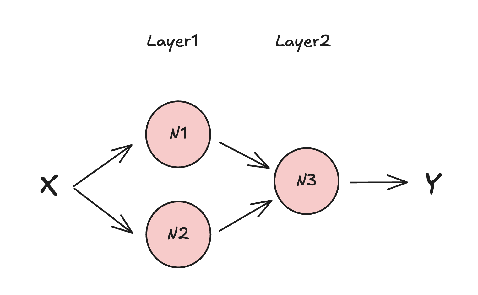
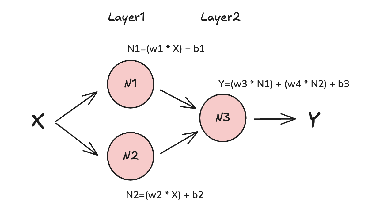
The diagram below illustrates a simple neural network with two layers and three neurons in total. The same input X is passed to both neurons in the first layer. These neurons process the input and forward their results to the second layer, where a single neuron performs the final computation, typically involving loss detection and calculation, to produce the output Y.

On the code level we would need to change the learning model definition as follows:

...snipped...
# Define the model
layer1 = keras.layers.Dense(units=2, input_shape=[1]) # input_shape is defined only for the first layer
layer2 = keras.layers.Dense(units=1) # automatically gets inputs from the previous layer

model = keras.Sequential([layer1, layer2]) # 2 layers. 2 neurons in L1, 1 neuron in L2
...snippped...

…and the result would be more closer to 19:

...snipped...
Epoch 48/50
1/1 ━━━━━━━━━━━━━━━━━━━━ 0s 17ms/step - loss: 0.0343
Epoch 49/50
1/1 ━━━━━━━━━━━━━━━━━━━━ 0s 17ms/step - loss: 0.0321
Epoch 50/50
1/1 ━━━━━━━━━━━━━━━━━━━━ 0s 19ms/step - loss: 0.0300
1/1 ━━━━━━━━━━━━━━━━━━━━ 0s 24ms/step
[[18.552378]]

How does our original single-neuron function Y=(w * X) + b looks like in multi-neuron network?

Each neuron makes its own “guess” by assigning a weight and introducing a bias to the input it receives. The resulting output is then passed to the next neuron, which applies its own new weight and bias. This process continues through the network.

For example, the output might take the form: Y = (w3 * N1) + (w4 * N2) + b3

Here, N1 and N2 are the outputs from the previous layer’s neurons, w3 and w4 are the new weights, and b3 is the bias added by the last neuron.

While having a basic understanding of neural networks, we can extend our vocabulary a bit further: In the context of neural networks, a tensor is a general term for the data structures, such as inputs, outputs, and weights, that flow through the network. Tensors can have different dimensions, from simple scalars and vectors to complex multi-dimensional arrays.

You might also hear the term model parameters. These refer to a subset of tensors - specifically the weights and biases that the model learns and adjusts during training.

In our small examples, the model might have just a few dozen parameters. In contrast, large-scale models like Meta’s LLaMA or OpenAI’s ChatGPT have hundreds of millions or even trillions of parameters.

Complex neural networks

Neural networks can be far more complex than the simple examples we’ve seen so far and they’re typically characterized by several key features:

many layers
many neurons in each layer
neurons can talk to themselves or to the neurons in the same layer
neuron talk to a subset of neurons in the previous layer only
“activation” functions involved
multidimensional inputs and outputs
and many more…

The final computation at the end of a neural network will be a composition of inter-related convoluted functions. So far, this article assumed a “feedforward” Dense neural layers where each neuron talks to all neurons in the next layer - that is why “dense”, of fully connected network. Keras offers much more than that, it offers tens of layer types and even custom layers to build super-complex neural networks.

Training data

Machine learning (ML) models are only as good as the data they are trained on. To build a model that performs well, you need a strong training dataset, which is a collection of input data paired with the expected outputs.

But training is just the beginning. Once your model has been trained, it is crucial to validate and test it to ensure it performs well on new, unseen data. This is why it is standard practice to split your dataset: one part for training, and another for validation (and possibly a third for testing). This helps you check if the model can generalize, rather than just memorize the training data - a problem known as overfitting.

Preparing well-normalized datasets is a topic of its own. Fortunately, TensorFlow Datasets provides a wide range of ready-to-use datasets, which can be easily loaded through the keras API we have been using.

Data classification

These datasets span various data types, like text, audio, images, and more. While the format of the data may differ, all datasets have one thing in common: they contain both data and labels. The data might be an encoded MP3 snippet, a handwritten character, or any other input, while the label is a human-readable tag that helps categorize the input. For example, if we are training a model to recognize spoken words, we might use audio samples of the word “yes,” each labeled as yes. This tells the model that all these samples belong to the same class.

This process is called classification. We are teaching the model to group similar data into categories. For instance, a classification model might learn to recognize and group different songs by genre, such as rock or jazz.

Training on specific data types: Images

Let’s take a high-level look at how to train a model to recognize images of dogs.

First, the data needs to be normalized. This usually means scaling the image size and also pixel values so they fall within a consistent range (typically 0 to 1).

Next, we apply various filters over the image to help the model learn relationships between individual pixels.

A key part of image-based training is feature extraction. For dog recognition, for example, the model should learn to identify parts like legs, ears, eyes, or the torso. These features help the model understand what visually characterizes a “dog.”

Another important step is data augmentation. This involves applying transformations like rotation, flipping, or skewing—to the training images. Augmentation increases dataset diversity and helps the model generalize better, reducing the risk of overfitting.

Various machine learning functions, e.g. convolutions may represent or encode the dog and dog parts as follows:

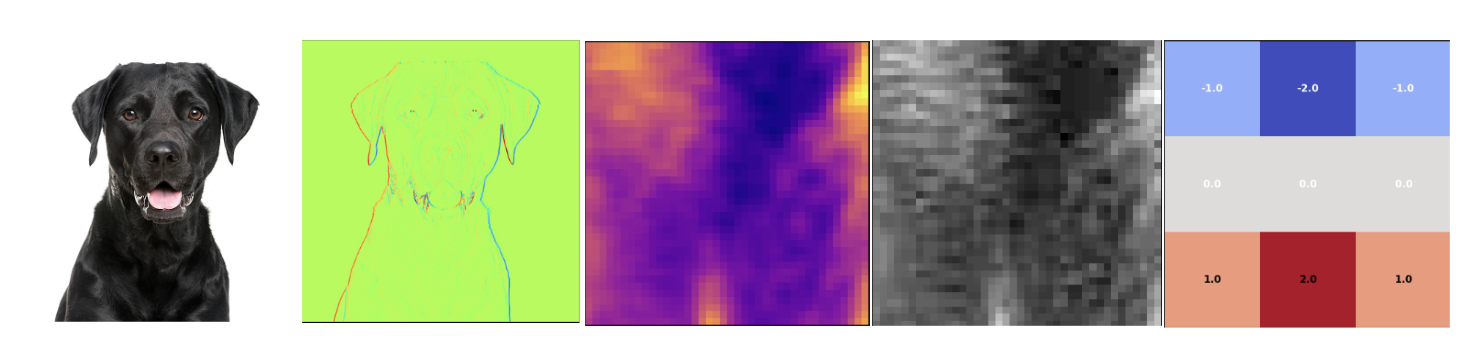
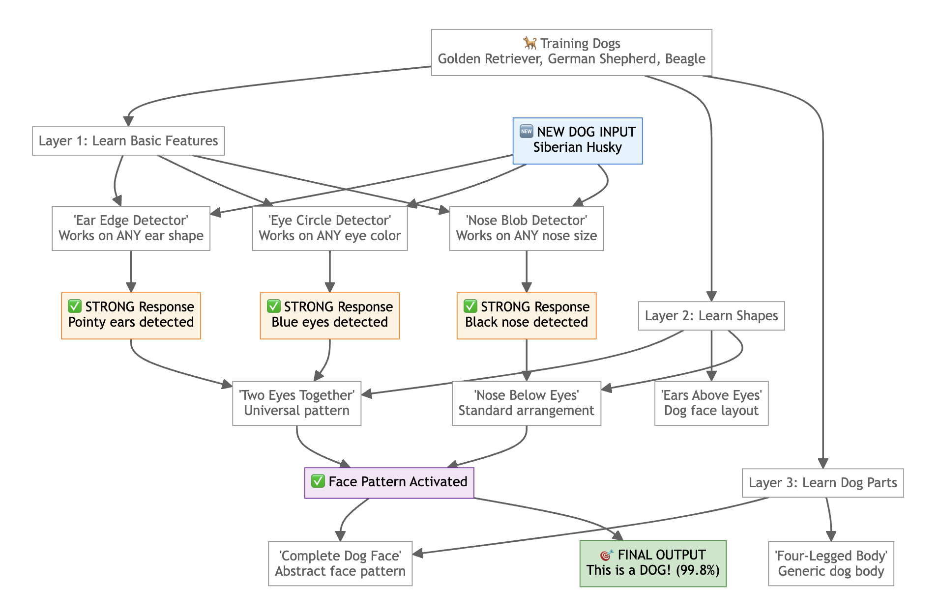
This kind of decomposition and transformation helps the model learn key visual characteristics that define a dog. For example:

The eyes are typically circular.
The ears are triangular and usually positioned above the eyes.
The nose appears below the eyes.
Four legs support the body structure.
The tongue’s color often stands out from the rest of the body.
…and many more subtle visual patterns.

These features, once extracted, allow the model to build a more accurate internal representation of what a “dog” looks like. When the model is trained properly, any dog image should fit in and will be properly classified. The prediction may look as follows:

If you would like to dive deeper into image processing, take a look at the this code. It builds on the concepts we’ve covered so far and uses TensorFlow to:

Load a pre-built image dataset
Normalize the data for efficient learning
Train the model
Validate the results
Convert the model to TFLite format for use on the microcontrollers
Save the trained model for offline use

This example will help solidify your understanding of how image classification works in practice.

Keyword spotting

Another very popular daily-use example is keyword spotting, used in many home devices. Think of Alexa or Siri. When you say “Hey Google” or “Hey Siri”, the machine responds, because it has deteted some wake words. This concept is oftentimes used in low-performance TinyML models and is extetended by further cascaded process towards the cloud which works as follows:

User says “Hey Google”.
TinyML model with very low latency recognises a keyword.
Microcontroller records the subsequent words.
Subsequent words are passed to the cloud for more heavy processing in a full speech-recognition model.
User is provided with a full response.

Keyword spotting might sound like a trivial task, but it is actually quite complex. Just like with image recognition, sound data must be carefully processed and decomposed before it can be used to train a model effectively.

It is not enough to simply record audio samples and analyze the raw waveforms by looking at their amplitudes or shapes. Even very different words—like “yes” and “no” can appear surprisingly similar when represented as basic sound waves. Without proper preprocessing, the model may struggle to reliably distinguish them.

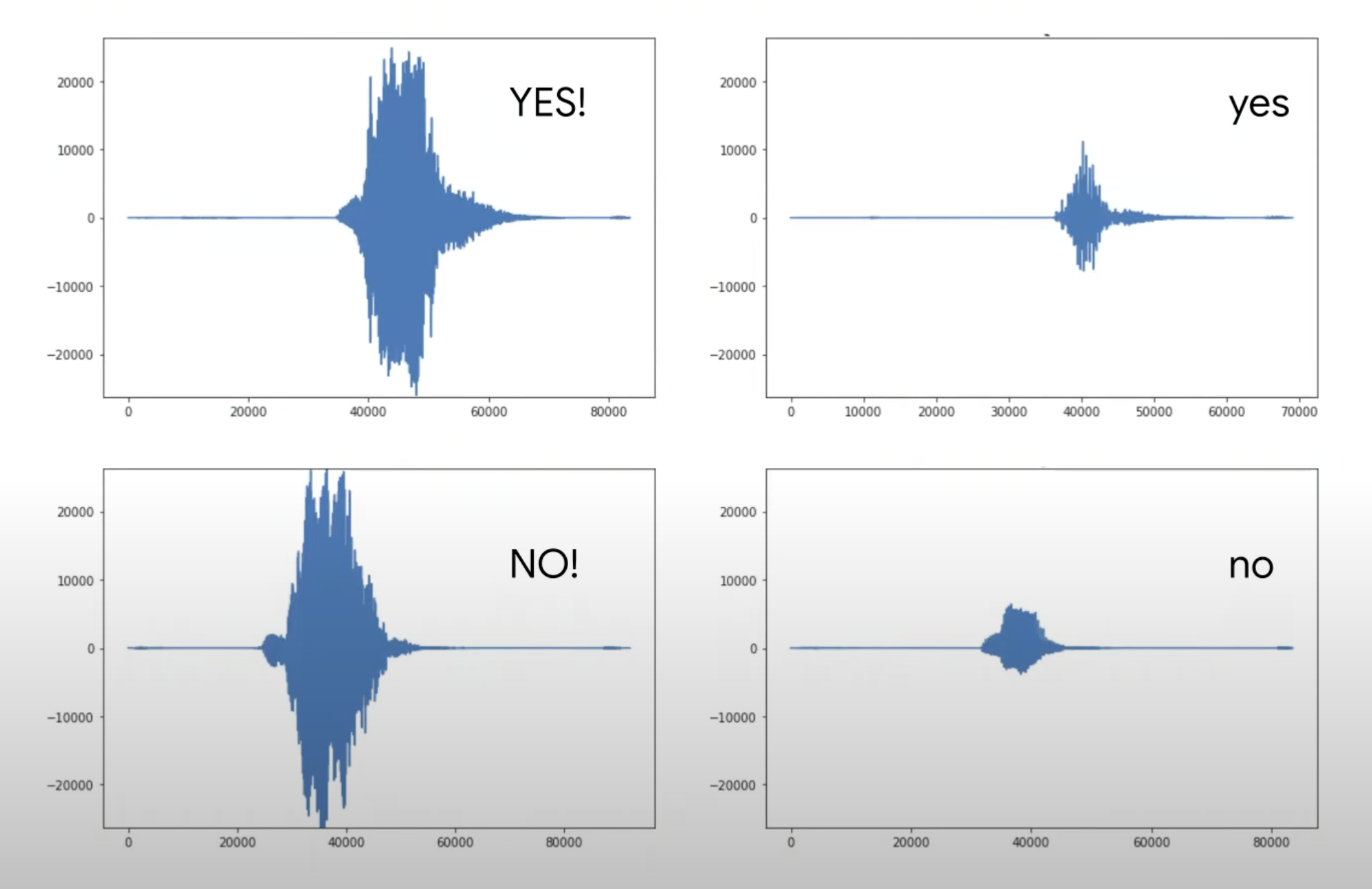
Typical sound wave preprocessing technique Fourier transform - being one of many. Sound waves are decomposed and unique characteristics and features are emphasised:

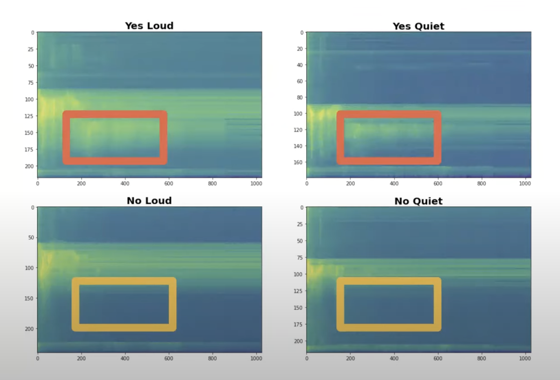
Even minimalistic Micro Speech model has 49 spectrographic features, each feature consisting of 40 channels of data.

Anytime Alexa hears a new sound, it runs the input through various transformations in the neural network to classify the words properly.

Rule your laptop by voice commands.

Now let’s turn the theory into the code and let your voice command your computer.

To avoid reinventing the wheel (and, more importantly, to save hours of data collection and model tuning), we can take advantage of work already done by the ML community:

Use pre-recorded audio samples, e.g. Google’s Speech Commands dataset with tens of thousands voice samples of dozens of english words.
Reuse pre-trained models, e.g. from Hugginface. Brave ones can train by themselves though.

Using Pre-trained Hugging Face Models

Let’s see just how easy it is to use a pre-trained keyword spotting model in practice. The wav2vec2-base-ft-keyword-spotting model achieves impressive 98.26% accuracy and can recognize 12 different keywords: “yes”, “no”, “up”, “down”, “left”, “right”, “on”, “off”, “stop”, “go”, plus silence and unknown classes.

See a ready-to-use Python code that listens for a voice command and opens your browser (in this case, Chrome on macOS) when it hears the word “go”. This is the same example demonstrated in the video at the beginning of this post.

Closing words

Neural networks might seem intimidating at first, but even simple models can produce powerful applications like voice-activated actions. As we have seen, understanding the core building blocks (neurons, weights, biases, tensors, and layers) helps demystify the “magic” behind AI and ML.

What I have covered here is just the surface, a simplified view meant to explain the core mechanics of neural networks. Behind the scenes of today’s advanced AI systems are teams solving problems that span mathematics, data engineering, distributed systems, and human-centered design.

While studying this topic, I gained a new level of appreciation for the people building state-of-the-art AI systems. It is one thing to understand a basic neural network, but designing, training, and scaling the models behind tools like ChatGPT or LLaMA is something entirely different.

Tags:
AI